Introduction
This method is developed for a determination of a plasma-membrane affinity of proteins which are significantly localised in both plasma membrane and cytoplasm, typically peripherally-associated plasma-membrane proteins.
This method enables an exact determination of a distribution ratio between a plasma-membrane and a cytoplasmic fraction and is very useful for investigation of an point-mutation effect on protein localisation.
A determining is based on single confocal images and omits sophisticated imaging methods.
Why this method
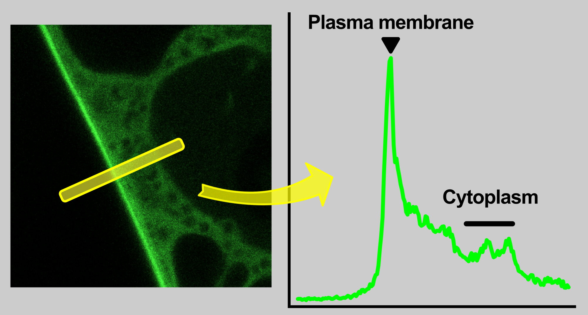
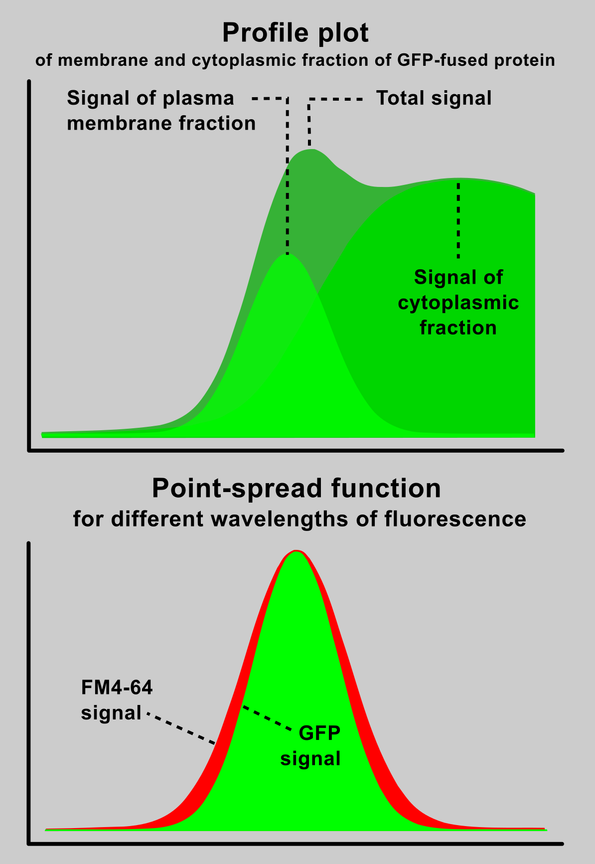
An intuitive way to compare a plasma-membrane and a cytoplasmic fraction of a fluorescently-tagged protein is to perform a linear profile, which is a standard function of ImageJ software.
By a simple approach, the maximum of a plasma-membrane peak and average cytoplasmic fluorescence intensity are taken for a profile data quantification. As we describe bellow, but this practice can give a relevant result only when membrane intensity is distinctly greater then cytoplasmic.
Nature of confocal signal
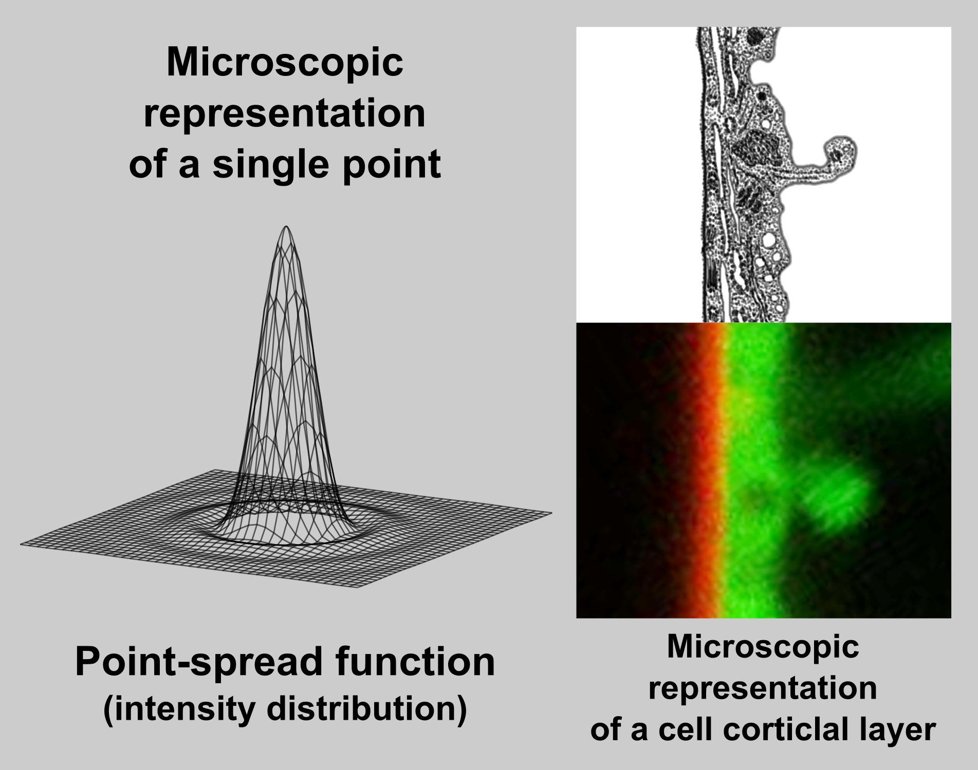
In fact, an image captured by a (confocal) microscope is only a sum of diffraction patterns. Each point-source of an original object is imaged according to Airy point-spread function (left) and the resulting image is given by superposition of this particular distribution.
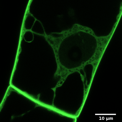
On example image (right, bottom) is a cortical region of a Green fluorescent protein (GFP) expressing plant cell, which is labelled by FM4-64 dye. FM4-64 is a red marker of plasma membrane and GFP acts as a green cytoplasmic marker. Image was captured by a laser confocal microscope with a 63x 1.4NA water immersion objective. You can compare a relatively wide (~ 400 nm) band of plasma membrane, which real thickness is about 10 nm (idealised picture right, above).
Source of image: Wikipedia.
Complications of membrane signal measurement
- A fluorescence intensity at the position of plasma membrane (defined by FM4-64 marker) is not equal to the true signal emitted by a plasma-membrane associated fraction of the GFP-tagged protein. Due to diffraction phenomena, the cytoplasmic signal is spread over the plasma-membrane region. When the cytoplasmic fraction of the protein is more dominant than the plasma-membrane fraction, a plasma-membrane localisation determined from a measurement of fluorescence intensity at the plasma-membrane position considerably overestimate the real state.
- The maximum of the tagged-protein fluorescence signal does not co-localise with the position of plasma membrane. Because the measured signal is a result of superposition of the plasma-membrane and the cytoplasmic compounds, its maximum is typically shifted towards the cytoplasm.
- Peak of a plasma-membrane marker FM4-64 cannot be used as a mask for a membrane signal selection Firstly, a cytoplasmic signal is included in the region delimited by FM4-64 peak, and secondly, due to the wavelength-dependency of a point-spread function, the red FM4-64 peak is wider than the green peak of a GFP-tagged protein.
Principle of method
Decomposition of measured fluorescence
Our approach is based on a decomposition of a fluorescence profile of a peripherally-associated plasma-membrane protein into a plasma-membrane and a cytoplasmic compounds according to a model of fluorescence signal distribution.
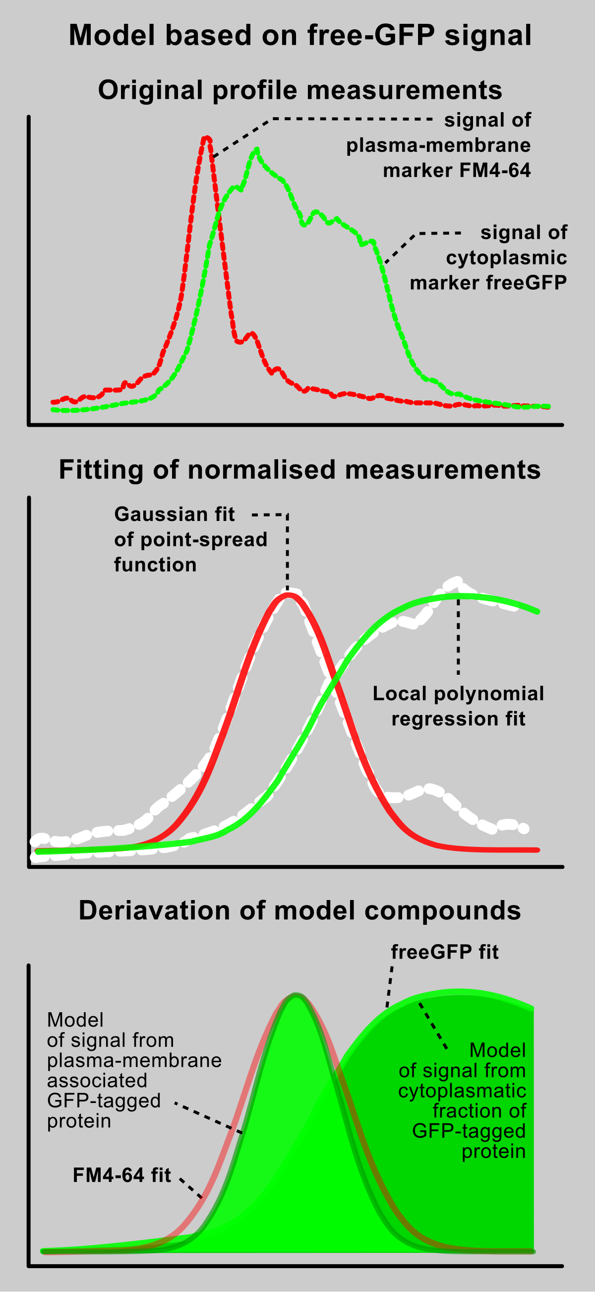
The model is created from profile measurements acquired from cells expressing a cytoplasmic marker, which are also labelled by plasma-membrane marker dye. Cytoplasmic marker must have same fluorochome as used for visualisation of the examined peripheral protein.
When GFP is used for a protein tagging, free-GFP or a purely cytoplasmic GFP-tagged protein could be used as cytoplasmic markers. For a labelling of plasma membrane, a red fluorescence emitting styryl dye FM4-64 is the optimal choice. Fluorescently-labelled membrane proteins can be also used, but their strict plasma-membrane localisation must be confirmed.
Model creation
Profiles of a cytoplasmic marker are normalised, joined and fitted by a local polynomial regression. The resulting fit is returned as the model of cytoplasmic compound of fluorescence signal.
A plasma-membrane marker signal is assumed as a point-source signal and is fitted by a Gaussian form of the point spread function:
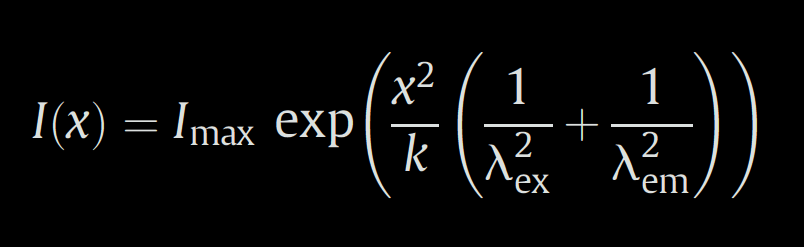
where x is x-coordinate of the profile measurement, λex and λem are marker excitation and emission wavelengths respectively, k is a constant depending on an numerical aperture of the used objective and I(x) and Imax are fluorescence intensities. Parameters k and Imax are optimised by non-linear least square (nls) method.
An ideal course of function of point-spread function for a fluorochrome used for a visualisation of the tested peripheral protein is derived from this Gaussian fit. Parameters λex and λem are set with respect to the used fluorochrome and k is taken from the fitting. Imax is set equal to 1 for a normalised distribution.

Analysis of measurements
The fluorescence distributions of tested peripherally-associated plasma-membrane proteins are decomposed into the plasma-membrane and the cytoplasmic compound using non-linear least square fitting.
Prior to the fitting, the real position of plasma membrane in profiles is determined from the maximum of fluorescence signal of a plasma-membrane marker. The maximum is identified on transformed marker signal, which was smoothed by a local polynomial regression. The x-coordinate of the plasma membrane position in the profile is then set to zero.
The x-transformed fluorescence signal IGFP(x) is fitted by the formula:
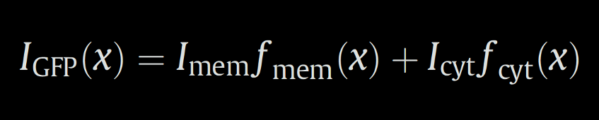
where fmem(x) and fcyt(x) are the model components describing a course of function for the membrane and the cytoplasmic fluorescence distribution respectively, and Imem and Icyt are intensities of each compound, which are optimised by the fitting.
The total amount of the plasma-membrane associated fluorescence Φmem is calculated by the integration of the fitted plasma membrane compound according thε formula

The plasma membrane affinity ξmem/cyt of the tested protein is defined as

where Φmem is equal to the total amount of the labelled protein in the patch of the plasma membrane examined by the profile and Icyt is equal to the average cytoplasmic protein concentration in a three-dimensional shape delimited by the length, the width and the thickness of the profile. The ξmem/cyt parameter is in fact the length of the profile, in which is the same amount of the protein as in the adjacent patch of the plasma membrane.
The lowest image shows an example of the analysis results. A GFP-tagged intrinsic plasma membrane protein PMA1 (Plasma-membrane ATPase 1), cytoplasmic free GFP protein and peripherally-associated plasma-membrane protein DREPP2 (Developmentally-regulated plasma-membrane polypeptide 2) from tobacco was expressed in tobacco BY-2 suspension cells. The box-plots clearly show a very high plasma-membrane affinity of intrinsic protein and a slightly lower affinity of peripheral protein in contrast with purely cytoplasmic GFP. The fourth plot shows the lowered plasma-membrane affinity of DREPP2 protein carrying a mutation in myristoylation site. This mutation is responsible for detachment of the protein from plasma membrane.
How to collect images
For the analysis, two-channel single-slice confocal images with a high-resolution are required:
- a colour depth: 12-16 bit
- a resolution: 15 px/μm and more
- plasma membrane must be perpendicular to the focal plain
- first channel: a fluorescently-tagged examined protein for analysis itself, cytoplasmic marker tagged by the same fluorophore (e.g. GFP) for the calibration.
- second channel: a plasma-membrane marker (e.g. FM4-64 dye)
Image analysis
Detailed tutorial was published in JoVE (Journal of Visualized Experiments)
ImageJ macro
Download an ImageJ macro Peripheral_.ijm
INSTALLATION: select Plugins | Macros | Install... in the main FIJI/ImageJ menu and specify the path to the downloaded file “Peripheral_.ijm.”
R source code and packages
INSTALLATION: Download the R package peripheral from source
and install them by selecting Packages | Install package(s) from local files... in R Gui menu.
Alternatively, run this command in R shell:
install.packages("http://kfrserver.natur.cuni.cz/lide/vosolsob/Peripheral/source/peripheral_latest.tar.gz", repo=NULL, type="source")
REQUIREMENTS: package ggplot2 is required, for instalation, run this command in R shell:
install.packages("ggplot2")
DOCUMENTATION: Full documentation to the package peripheral in PDF.
OTHER RELEASES: All version are deposited in this directory .
RELEASE NOTES: Actual version 2.2 - solved issue with import of ImageJ CSV file without index column.
Testing data
Download LIF calibration data for plain GFP localisation in BY-2 cells calibration.lif.
These pictures can be used for calibration in step 4.1 of JoVE tutorial.
Download LIF pictures of peripherally associated protein NtDREPP4 (with mutation S2A) in BY-2 cells DREPP4-S2A.lif
These pictures can be used for measurement in step 4.7 of JoVE tutorial.
Representative data from JoVE tutorial
BACKROUND: DREPP is plant peripherally associated protein. DREPP2 in Nicotiana tabacum is attached on the membrane by N-myristoylation on Gly2 and also by electrostatic interaction of poly-basic amino acid cluster (Lys-rich region) with phosphorylated phosphoinositides.
Mutation Gly2Ala (G2A) disrupts N-myristoylation and the electrostatic association can be affected by Wortmannin, inhibitor of phosphoinositides.
Measurement was calibrated using free GFP.
Creation of the model of PM & cytoplasmic distribution
Download representative CSV file with measurement of free GFP localisation for cytoplasmic signal calibration.
These data can be loaded directly in step 4.4 of JoVE tutorial (Plot profile) without previous work with images.
Run "Plot profile" macro, select import from 'Single file' and let 'Samples grouping factors' check-box unselected. You get this result:
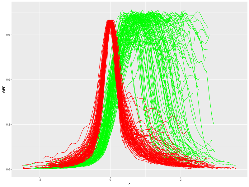
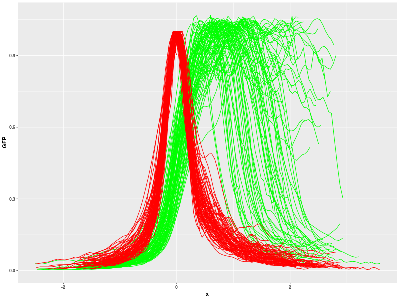
Using "Profile filtering setup" macro (step 4.5) with this setting:
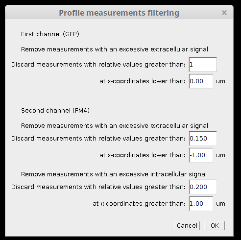
you can get cleaner results without excessive curves:
Now, you can continue "Create model" macro (step 4.6). Check 'Use filtering' and select data for analysis from 'Single file' (then select the file "cyto.csv" in dialog window). You get this result:
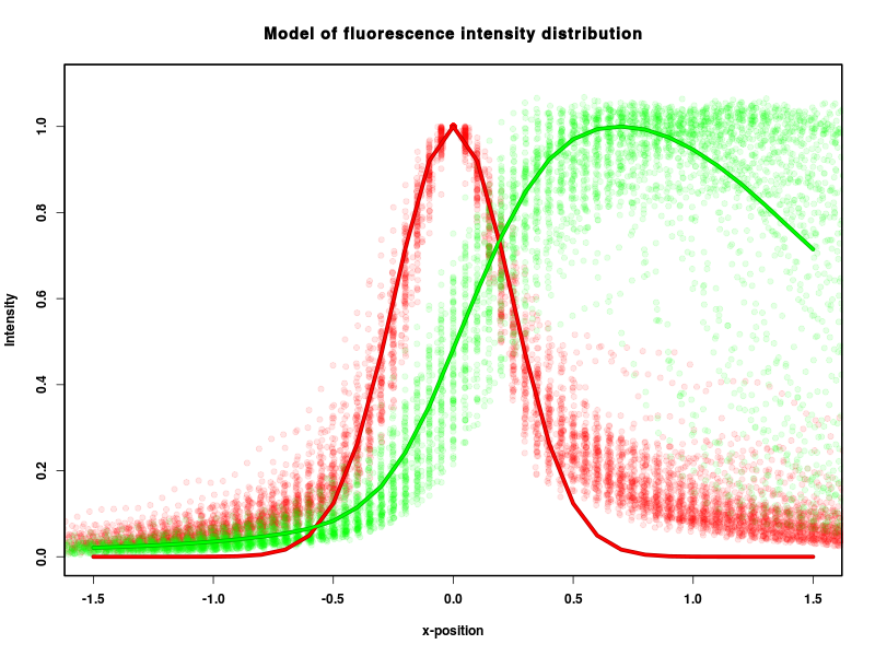
Model is stored in the file model.RData, which can be downloaded and used in following analysis without performing the calibration steps.
Data analysis
Download measurements of DREPP2 and DREPP2(G2A) localisation in normal conditions and after Wortmannin treatment.
These data can be loaded directly in the step 4.7 of JoVE tutorial. Save downloaded files in directory with any other CSV files and run "Plot profile" macro with 'Fac_0' and 'Fac_1' selected (plots will be created by all variants) and select option 'All files in directory'. Then select the directory with downloaded files in dialog windows. You get this results:
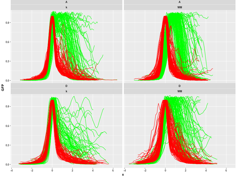
The profile filtering is also recommended now. You can clean data:

Now proceed to "Calculate distribution" macro (step 4.8 of JoVE tutotial).
Set analysis according to this example:

The result will be presented as box-plot:

NOTE: During this analysis, new CSV file with results is being produced in your directory. If you start this analysis again with option 'All files in directory', analysis crashes. Please, remove result file or change its suffix to e.g. ".xlsx" or ".txt".
How to cite this method
This method was originally described in Vosolsobě S., Petrášek J., Schwarzerová K. (2017): Evolutionary plasticity of plasma membrane interaction in DREPP family proteins. Biochimica et Biophysica Acta (BBA)-Biomembranes 1859 (5), 686-697
Detailed protocol was published in Vosolsobě, S., Schwarzerová, K., Petrášek, J. (2018): Determination of Plasma Membrane Partitioning for Peripherally-associated Proteins. JoVE (Journal of Visualized Experiments) (136), e57837
Contact
Developed by Stanislav Vosolsobě, Charles University, Prague, Czech Republic
Please, contact me on e-mail vosolsob@natur.cuni.cz